Heys Its all about my Project

Location Tracking Approaches

Cell of Origin

Distance-Based (Lateration) Techniques

Time of Arrival

Time Difference of Arrival (TDoA)

Received Signal Strength (RSS)

Angle-Based (Angulation) Techniques

Angle of Arrival (AoA)

Location Patterning (Pattern Recognition) Techniques

Calibration Phase

Operational Phase

Location Tracking Approaches

Location tracking and positioning systems can be classified by the measurement techniques they employ to determine mobile device location (localization). These approaches differ in terms of the specific technique used to sense and measure the position of the mobile device in the target environment under observation. Typically, Real Time Location Systems (RTLS) can be grouped into four basic categories of systems that determine position on the basis of the following:

•

Cell of origin (nearest cell)

•

Distance (lateration)

•

Angle (angulation)

•

Location patterning (pattern recognition)

An RTLS designer can choose to implement one or more of these techniques. This may be clearly seen in some approaches that attempt to optimize performance in two or more environments with very different propagation characteristics. The popularity of this approach is such that it is often not unusual to hear arguments supporting the case for a fifth category that encompasses RTLS offerings that sense and measure position using a combination of at least two of these methods.

Keep in mind that regardless of the underlying positioning technology, the "real-time" nature of an RTLS is only as real-time as its most current timestamps, signal strength readings, or angle-of-incidence measurements. The timing of probe responses, tag transmissions, and location server polling intervals can introduce discrepancies between the actual and reported device position observed during each reporting interval.

Cell of Origin

One of the simplest mechanisms of estimating approximate location in any system based on RF "cells" is the concept of cell-of-origin (or "associated access point" in Wi-Fi 802.11 systems), as shown in Figure 2-1.

Figure 2-1 Cell of Origin

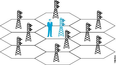
In its simplest form, this technique makes no explicit attempt to resolve the position of the mobile device beyond indicating the cell with which the mobile device is (or has been) registered. When applied to 802.11 systems, this technique tracks the cell to which a mobile device associates. The primary advantage of this technique is ease of implementation. Cell of origin does not require the implementation of complicated algorithms and thus positioning performance is very fast. Almost all cell-based WLANs and other cellular-based RF systems can be easily and cost-effectively adapted to provide cell of origin positioning capability. However, the overwhelming drawback of pure cell of origin positioning approaches continues to be coarse granularity. For various reasons, mobile devices can be associated to cells that are not in close physical proximity, despite the fact that other nearby cells would be better candidates. This coarse granularity can be especially frustrating when attempting to resolve the actual location of a mobile device in a multi-story structure where there is considerable floor-to-floor cell overlap.

To better determine which areas of the cell possess the highest probability of containing the mobile device, some additional method of resolving location within the cell is usually required. This can either be a manual method (such as a human searching the entire cell for the device) or a computer-assisted method. When receiving cells provide received signal strength indication (RSSI) for mobile devices, the use of the highest signal strength technique can improve location granularity over the cell of origin. In this approach, the localization of the mobile device is performed based on the cell that detects the mobile device with the highest signal strength. This is shown in Figure 2-2, where the blue rectangular client device icon is placed nearest the cell that has detected it with the highest signal strength.

Figure 2-2 Highest Signal Strength Technique

Using this technique, the probability of selecting the true "nearest cell" is increased over that seen with pure cell of origin. Depending on the accuracy requirements of the underlying business application, performance may be more than sufficient for casual location of mobile clients using the highest signal strength technique. For instance, users intending to use location-based services only when necessary to help them find misplaced client devices in non-mission critical situations may be very comfortable with the combination of price and performance afforded by solutions using the highest signal strength approach. However, users requiring more precise location would find the inability of the highest signal strength technique to isolate the location of a mobile device with finer granularity than that of an entire coverage cell to be a serious limitation. These users are better served by those approaches using the techniques of lateration, angulation, and location patterning that provide finer resolution and improved accuracy. These techniques are discussed in subsequent sections.

Distance-Based (Lateration) Techniques

Time of Arrival

Time of Arrival (ToA) systems are based on the precise measurement of the arrival time of a signal transmitted from a mobile device to several receiving sensors. Because signals travel with a known velocity (approximately the speed of light (c) or ~300 meters per microsecond), the distance between the mobile device and each receiving sensor can be determined from the elapsed propagation time of the signal traveling between them. The ToA technique requires very precise knowledge of the transmission start time(s), and must ensure that all receiving sensors as well as the mobile device are accurately synchronized with a precise time source.

From knowledge of both propagation speed and measured time, it is possible to calculate the distance (D) between the mobile device and the receiving station:

D = c (t)

where:

•

D= distance (meters)

•

c = propagation speed of ~ 300 meters / microsecond

•

t = time in microseconds

With distance used as a radius, a circular representation of the area around the receiving sensor can be constructed for which the location of the mobile device is highly probable. ToA information from two sensors resolves a mobile device position to two equally probable points. ToA tri-lateration makes use of three sensors to allow the mobile device location to be resolved with improved accuracy.

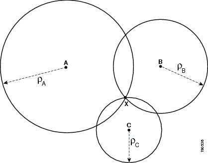
Figure 2-3 illustrates the concept of ToA tri-lateration. The amount of time required for a message transmitted from station X to arrive at receiving sensors A, B, and C is precisely measured as tA, tB, and tC. Given a known propagation velocity (stated as c), the mobile device distance from each of these three receiving sensors can then be calculated as DA, DB, and DC, respectively. Each calculated distance value is used to construct a circular plot around the respective receiving sensor. From the individual perspective of each receiver, station X is believed to reside somewhere along this plot. The intersection of the three circular plots resolves the location of station X as illustrated in Figure 2-3. In some cases, there may be more than one possible solution for the location of mobile device station X, even when using three remote sensors to perform tri-lateration. In these cases, four or more receiving sensors are employed to perform ToA multi-lateration.

Figure 2-3 Time of Arrival (ToA)

ToA techniques are capable of resolving location in two-dimensional as well as three-dimensional planes. 3D resolution can be performed by constructing spherical instead of circular models.

A drawback of the ToA approach is the requirement for precise time synchronization of all stations, especially the mobile device (which can be a daunting challenge for some 802.11 client device implementations). Given the high propagation speeds, very small discrepancies in time synchronization can result in very large errors in location accuracy. For example, a time measurement error as small as 100 nanoseconds can result in a localization error of 30 meters. ToA-based positioning solutions are typically challenged in environments where a large amount of multipath, interference, or noise may exist.

The Global Positioning System (GPS) is a example of a well-known ToA system where precision timing is provided by atomic clocks.

Time Difference of Arrival (TDoA)

Time Difference of Arrival (TDoA) techniques use relative time measurements at each receiving sensor in place of absolute time measurements. Because of this, TDoA does not require the use of a synchronized time source at the point of transmission (i.e. the mobile device) in order to resolve timestamps and determine location. With TDoA, a transmission with an unknown starting time is received at various receiving sensors, with only the receivers requiring time synchronization.

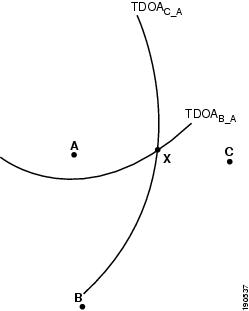
TDoA implementations are rooted upon a mathematical concept known as hyperbolic lateration. In this approach, at least three time-synchronized receiving sensors are required. In Figure 2-4, assume that when station X transmits a message, this message arrives at receiving sensor A with time TA and at receiving station B with time TB. The time difference of arrival for this message is calculated between the locations of sensors B and A as the positive constant k, such that:

TDoAB-A = | TB - TA | = k

The value of TDoAB-A can be used to construct a hyperbola with foci at the locations of both receiving sensors A and B. This hyperbola represents the locus of all the points in the x-y plane, the difference of whose distances from the two foci is equal to k(c) meters. Mathematically, this represents all possible locations of mobile device X such that:

| DXB - DXA | = k(c)

The probable location of mobile station X can then be represented by a point along this hyperbola. To further resolve the location of station X, a third receiving sensor at location C is used to calculate the message time difference of arrival between sensors C and A, or:

TDoAC-A = | TC - TA | = k1

Knowledge of constant k1 allows for the construction of a second hyperbola representing the locus of all the points in the x-y plane, the difference of whose distances from the two foci (that is, the two receiving sensors A and C) is equal to k1(c) meters. Mathematically, this can be seen as representing all possible locations of mobile device X such that:

| DXC - DXA | = k1(c)

Figure 2-4 illustrates how the intersection of the two hyperbolas TDoAC-A and TDoAB-A is used to resolve the position of station X.

Figure 2-4 Time Difference of Arrival (TDoA)

A fourth receiving sensor and third hyperbola may be added as an enhancement to perform TDoA hyperbolic multi-lateration. This may be required to solve for cases where there may be more than one solution when using TDoA hyperbolic tri-lateration.

Modern TDoA system designers have derived methods of coping with local clock oscillator drift that are intended to avoid the strict requirement for precision time synchronization of TDoA receivers. For example, time adjustments can be calculated periodically with regard to a reference clock source. These clock adjustments can then be used to correct for offsets from the reference clock elsewhere in the system. In the case of TDoA receivers that are capable of transmitting packets (for example, a TDoA receiver that may be integrated into an 802.11 WLAN access point), another innovative approach may involve the periodic exchange of "timing" packets between receivers. In this approach, time offsets between each receiver and a "reference receiver" can be quantized, with the resulting time adjustment applied accordingly within the system.

Airport ranging systems are a well-known example of TDoA systems in use today. In the world of cellular telephony, TDoA is also referred to as Enhanced Observed Time Difference (E-OTD), and in this specific application offers an outdoor accuracy in that application of about 60 meters in rural areas and 200 meters in RF-heavy urban areas.

ToA and TDoA have several similarities. Both have proven to be highly suitable for large-scale outdoor positioning systems. In addition, good results have been obtained from ToA and TDoA systems in semi-outdoor environments such as amphitheaters and stadiums, as well as contained outdoor environments such as car rental and new car lots or ports of entry. Indoors, TDoA systems exhibit their best performance in buildings that are large and relatively open, with low levels of overall obstruction and high ceilings that afford large areas of clearance between building contents and the interior ceiling. It is precisely in these open, spacious environments that TDoA and ToA-based systems operate at their peak efficiency and performance.

Received Signal Strength (RSS)

Thus far we have discussed two lateration techniques (ToA and TDoA) that use elapsed time to measure distance. Lateration can also be performed by using received signal strength (RSS) in place of time. With this approach, RSS is measured by either the mobile device or the receiving sensor. Knowledge of the transmitter output power, cable losses, and antenna gains as well as the appropriate path loss model allows you to solve for the distance between the two stations.

The following is an example of a common path loss model used for indoor propagation:

In this model:

•

PL represents the total path loss experienced between the receiver and sender in dB. This will typically be a value greater than or equal to zero.

•

PL1Meter represents the reference path loss in dB for the desired frequency when the receiver-to-transmitter distance is 1 meter. This must be specified as a value greater than or equal to zero.

•

d represents the distance between the transmitter and receiver in meters.

•

n represents the path loss exponent for the environment.

•

s represents the standard deviation associated with the degree of shadow fading present in the environment, in dB. This must be specified as a value greater than or equal to zero.

Path loss (PL) is the difference between the level of the transmitted signal, measured at face of the transmitting antenna, and the level at of the received signal, measured at the face of the receiving antenna. Path loss does not take antenna gains or cable losses into consideration. Path loss represents the level of signal attenuation present in the environment due to the effects of free space propagation, reflection, diffraction, and scattering.

The path loss exponent (n) indicates the rate at which the path loss increases with distance. The value of path loss exponent depends on frequency and environment, and is highly dependent on the degree of obstruction (or "clutter") present in the environment. Common path loss exponents range from a value of 2 for open free space to values greater than 2 in environments where obstructions are present. A typical path loss exponent for an indoor office environment may be 3.5, a dense commercial or industrial environment 3.7 to 4.0 and a dense home environment might be as high as 4.5.

The standard deviation of shadow fading (s) represents a measure of signal strength variability, (sometimes referred to as "noise") from sources that are not accounted for in the aforementioned path loss equation. This include factors such as attenuation due to the number of obstructions present, orientation differences between location receiver antennas and the antennas of client devices, reflections due to multipath, and so on. Diversity antenna implementations reduce perceived signal variation due to shadow fading, and for this reason diversity antennas are almost universally recommended. In many indoor installations using diversity antennas, the standard deviation of shadow fading is often seen between 3 and 7 dB.

The generally accepted method to calculate receiver signal strength given known quantities for transmit power, path loss, antenna gain, and cable losses is as follows:

RXPWR = TXPWR - LossTX + GainTX - PL + GainRX - LossRX

We can directly substitute our equation for path loss into the equation above. This enables us to solve for distance d as follows:

where the meaning of the terms in the equation above are:

•

RxPWR represents the detected receive signal strength in dB.

•

TxPWR represents the transmitter output power in dB.

•

LossTX represents the sum of all transmit-side cable and connector losses in dB.

•

GainTX represents the transmit-side antenna gain in dBi.

•

LossRX represents the sum of all receive-side cable and connector losses in dB.

•

GainRX represents the receive-side antenna gain in dBi.

Note that all of these are to be specified as positive values.

Solving for distance between the receiver and mobile device allows a circular area to be plotted around the location of the receiver, using the distance d as the radius. The location of the mobile device is believed to be somewhere on this circular plot. As in other techniques, input from other receivers in other cells (in this case, signal strength information or RSSI) can be used to perform RSS tri-lateration or RSS multi-lateration to further refine location accuracy.

The signal strength information used to determine position can be obtained from one of two sources:

•

The network infrastructure reporting the received signal strength at which it receives mobile device transmissions ("network-side")

•

The mobile device reporting the signal strength at which it receives transmissions from the network ("client-side")

In 802.11 WLANs, the granularity with which RSSI is reported typically varies from radio vendor to radio vendor. In fact, 802.11 client devices produced by different silicon manufacturers may report received signal strength using inconsistent metrics. This can result in degraded and inconsistent location tracking performance. Location tracking solutions that utilize "network-side" RSSI measurements avoid this potential pitfall when supporting mobile devices from various manufacturers, since all measurement of RSSI is performed at the network infrastructure, not at the mobile device. This is a straightforward approach and is approach most often implemented by vendors of RSS lateration solutions, since a much higher degree of control is typically exercised over consistency in network infrastructure versus end user client mobile devices.

Location tracking solutions that rely on "client-side" RSSI measurements must take extra steps to avoid location inaccuracies that may be due to inconsistent mobile device hardware. Since it is not realistic to assume that every mobile device will be provided by the same hardware vendor, a method of "equalizing" any variations in relation to some assumed "reference model" is necessary. For example, assume that a particular positioning system expects to see reported RSSI in a range from -127dBm to +127dBm in 254 increments of 1 dBm each. Mathematical compensation will be required if only some mobile devices in the system can support this expectation (for example, other devices in the system may only be able to report RSSI in a range from -111dBm to +111 dBm in 74 increments of 3dBm each).

Typically, the responsibility for providing such equalization lies with the provider of the location solution. It is common to see such adjustments made through proprietary client software that installed on each mobile device in order to ensure all mobile devices can be located with approximate equal consistency.

To date, implementations using RSS lateration have enjoyed a cost advantage by not requiring specialized hardware at the mobile device or network infrastructure locations. This makes signal strength-based lateration techniques very attractive from a cost-performance standpoint to designers of 802.11-based WLAN systems wishing to offer integrated lateration-based positioning solutions. However, a known drawback to "pure" RSS lateration is that propagation anomalies brought about by anisotropic conditions in the environment may degrade accuracy significantly. This is due in part because in reality, propagation in any cell is far from a purely circular pattern based on an ideal path loss model. "Textbook" theoretical RSS lateration models in their purest form do not provide for the measurement or consideration of variations seen within actual sites, typically assuming only well-known values for path loss and shadow fading.

Pure RSS-based lateration techniques that do not take additional steps to account for attenuation and multipath in the environment rarely produce acceptable results except in very controlled situations. This includes those controlled situations where there is always established clear line-of-sight between the mobile device and the receiving sensors, with little attenuation to be concerned other than free-space path loss and minor impact from multipath.

Angle-Based (Angulation) Techniques

Angle of Arrival (AoA)

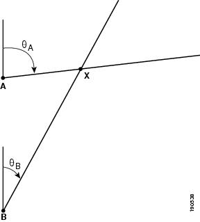
The Angle of Arrival (AoA) technique, sometimes referred to as Direction of Arrival (DoA), locates the mobile station by determining the angle of incidence at which signals arrive at the receiving sensor. Geometric relationships can then be used to estimate location from the intersection of two lines of bearing (LoBs) formed by a radial line to each receiving sensor, as illustrated in Figure 2-5. In a two-dimensional plane, at least two receiving sensors are required for location estimation with improved accuracy coming from at least three or more receiving sensors (triangulation).

Figure 2-5 Angle of Arrival (AoA)

In its purest form (that is, where clear line-of-sight is evident between the mobile device X and receiving sensors A and B), mechanically-agile directional antennas deployed at the receiving sensors are adjusted to the point of highest signal strength. The positioning of the directional antennas can be directly used to determine the LoBs and measure the angles of incidence qA and qB.

In practical commercial and military implementations of AoA, multiple element antenna arrays are used to sample the receiving signal, thereby eliminating the need for more complex and maintenance-intensive mechanical antenna systems. Electronic switching can be performed between arrays or portions of each array, and mathematical computations handled by a background computing system used to extract the angles of incidence. This technique actually involves calculating TDoA between elements of the array by measuring the difference in received phase at each element. In a properly constructed array, there is a small but discernible per element arrival time and a difference in phase. Sometimes referred to as "reverse beam-forming", this technique involves directly measuring the arrival time of the signal at each element, computing the TDoA between array elements, and converting this information to an AoA measurement. This is made possible because of the fact that in beam-forming, the signal from each element is time-delayed (phase shifted) to "steer" the gain of the antenna array.

A well-known implementation of AoA is the VOR (VHF Omnidirectional Range) system used for aircraft navigation from 108.1 to 117.95 MHz. VOR beacons around the United States and elsewhere transmit multiple VHF "radials" with each radial emanating at a different angle of incidence. The VOR receiver in an aircraft can determine the radial on which the aircraft is situated as it is approaching the VOR beacon and thus its angle of incidence with respect to the beacon. Using a minimum of two VOR beacons, the aircraft navigator is able to use onboard AoA ranging equipment to conduct angulation (or tri-angulation if using three VOR beacons) and accurately determine the position of the aircraft.

AoA techniques have also been applied in the cellular industry in early efforts to provide location tracking services for mobile phone users. This was primarily intended to comply with regulations requiring cell systems to report the location of a user placing an emergency (911) call. Multiple tower sites calculate the AoA of the signal of the cellular user, and use this information to perform tri-angulation. That information is relayed to switching processors that calculate the user location and convert the AoA data to latitude and longitude coordinates, which in turn is provided to emergency responder dispatch systems.

A common drawback that AoA shares with some of the other techniques mentioned is its susceptibility to multipath interference. As stated earlier, AoA works well in situations with direct line of sight, but suffers from decreased accuracy and precision when confronted with signal reflections from surrounding objects. Unfortunately, in dense urban areas, AoA becomes barely usable because line of sight to two or more base stations is seldom present.

Location Patterning (Pattern Recognition) Techniques

Location patterning refers to a technique that is based on the sampling and recording of radio signal behavior patterns in specific environments. Technically speaking, a location patterning solution does not require specialized hardware in either the mobile device or the receiving sensor (although at least one well-known location patterning-based RTLS requires proprietary RFID tags and software on each client device to enable "client-side" reporting of RSSI to its location positioning server). Location patterning may be implemented totally in software, which can reduce complexity and cost significantly compared to angulation or purely time-based lateration systems.

Location patterning techniques fundamentally assume the following:

•

That each potential device location ideally possesses a distinctly unique RF "signature". The closer to reality this assumption is, the better the performance of the location patterning solution.

•

That each floor or subsection possesses unique signal propagation characteristics. Despite all efforts at identical equipment placement, no two floors, buildings, or campuses are truly identical from the perspective of a pattern recognition RTLS solution.

Although most commercially location patterning solutions typically base such signatures on received signal strength (RSSI), pattern recognition can be extended to include ToA, AoA or TDoA-based RF signatures as well. Deployment of patterning-based positioning systems can typically be divided into two phases:

•

Calibration phase

•

Operation phase

During the operational phase, solutions based on location patterning rely on the ability to "match" the reported RF signature of a tracked device against the database of RF signatures amassed during the calibration phase. Because the database of recorded RF signatures is meant to be compiled during a representative period in the operation of the site, variations such as attenuation from walls and other objects can be directly accounted for during the calibration phase.

Calibration Phase

During the calibration phase, data is accumulated by performing a walk-around of the target environment with a mobile device and allowing multiple receiving sensors (access points in the case of 802.11 WLANs) to sample the signal strength of the mobile device (this refers to a "network-side" implementation of location patterning).

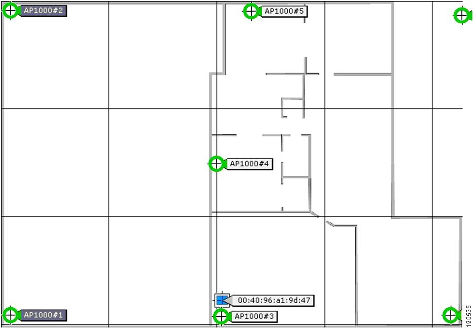
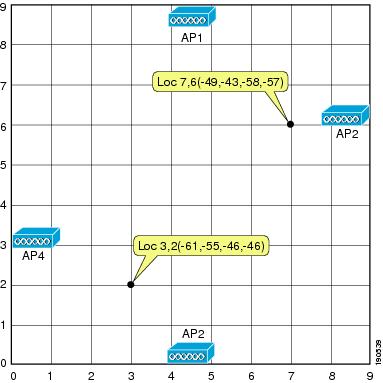
A graphical representation of the area to be calibrated is typically overlaid with a set of grid points or notations to guide the operator in determining precisely where sample data should be acquired. At each sample location, the array (or location vector) of RSS values associated with the calibration device is recorded into a database known as a radio map or training set. The size of the vector for this sample location is determined by the number of receiving stations that can detect the mobile device. Figure 2-6 provides a simplified illustration of this approach, showing two sample points and how their respective location vectors might be formed from detected client RSSI.

Figure 2-6 Location Patterning Calibration

Because of fading and other phenomena, the observed signal strength of a mobile device at a particular location is not static but is seen to vary over time. As a result, calibration phase software typically records many samples of signal strength for a mobile device during the actual sampling process. Depending on technique, the actual vector array element recorded may account for this variation via one or more creative approaches. A popular, simple-to-implement method is to represent the array element associated with any specific receiver as the mean signal strength of all measurements of that mobile device made by that receiver sensor for the reported sample coordinates. The location vector therefore becomes a vector array of mean signal strength elements as shown in the following equation, where x and y represent the reported coordinates of the sample and r represents the reported RSSI:

Operational Phase

In the operational phase, a group of receiving sensors provide signal strength measurements pertaining to a tracked mobile device (network-side reporting implementation) and forwards that information to a location tracking server. The location server uses a complex positioning algorithm and the radio map database to estimate the location of the mobile device. The server then reports the location estimate to the location client application requesting the positioning information.

Location patterning positioning algorithms can be classified into three basic groups:

•

Deterministic algorithms attempt to find minimum statistical signal distance between a detected RSSI location vector and the location vectors of the various calibration sample points. This may or may not be equal to the minimum physical distance between the actual device physical location and the recorded location of the calibration sample. The sample point with the minimum statistical signal distance between itself and the detected location vector is generally regarded as the best raw location estimate contained in the calibration database. Examples of deterministic algorithms are those based on the computation of Euclidean, Manhattan, or Mahalanobis distances.

•

Probabilistic algorithms use probability inferences to determine the likelihood of a particular location given that a particular location vector array has already been detected. The calibration database itself is considered as an a priori conditional probability distribution by the algorithm to determine the likelihood of a particular location occurrence. Examples of such approaches include those using Bayesian probability inferences.

•

Other techniques go outside the boundaries of deterministic and probabilistic approaches. One such approach involves the assumption that location patterning is far too complex to be analyzed mathematically and requires the application of non-linear discriminant functions for classification (neural networks). Another technique, known as support vector modeling or SVM, is based on risk minimization and combines statistics, machine learning, and the principles of neural networks.

To gain insight into how such location patterning algorithms operate, we can examine a simple example that demonstrates the use of a deterministic algorithm, which in this case will be the Euclidean distance. As stated earlier, deterministic algorithms compute the minimum statistical signal distance, which may or may not be equal to the minimum physical distance between the actual device physical location and the recorded location of the calibration sample.

For example, assume two access points X and Y and a mobile device Z. Access point X reports mobile device Z with an RSS sample of x1. Almost simultaneously, access point Y reports mobile device Z with an RSS sample of y1. These two RSS reports can be represented as location vector of (x1,y1). Assume that during the calibration phase, a large population of location vectors of the format F(x2,y2) were populated into the location server calibration database, where F represents the actual physical coordinates of the recorded location.

The location server can calculate the Euclidean distance d between the currently reported location vector (x1,y1) and each location vector in the calibration radio map as follows:

The physical coordinates F associated with the database location vector possessing the minimum Euclidean distance from the reported location vector of the mobile device is generally regarded as being the correct estimate of the position of the mobile device.

In a similar fashion to RSS lateration solutions, real-time location systems using location patterning typically allow vendors to make good use of existing wireless infrastructure. This can often be an advantage over AoA, ToA, and TDoA approaches, depending on the particular implementation. Location patterning solutions are capable of providing very good performance in indoor environments, with a minimum of three reporting receivers required to be in range of mobile devices at all times. Increased accuracy and performance (often well in excess of 5 meters accuracy) is possible when six to ten receivers are in range of the mobile device.

Location patterning applications perform well when there are sufficient array entries per location vector to allow individual locations to be readily distinguishable by the positioning application. However, this requirement can also contribute to some less-than-desirable deployment characteristics. With location patterning, achieving high performance levels typically requires not only higher numbers of receivers (or access points for 802.11) but also much tighter spacing. In large areas where it is possible for clients to move about almost anywhere, calibration times can be quite long. For this reason, some commercial implementations of location patterning allow the user to segment the target location environment into areas where client movement is likely and those where client movement is possible but significantly less likely, as well as areas where client location is impossible (such as within the thick walls of a tunnel, for example, or suspended within the open air space of an indoor building atrium). The amount of calibration as well as computational resources allocated to these two classes of areas is adjusted by the positioning application according to the relative probability of a client being located there.

The radio maps or calibration databases used by pattern recognition positioning engines tend to be very specific to the areas used in their creation, with little opportunity for re-use. The likelihood is very low that any two areas, no matter how identical they may seem in construction and layout, will yield identical calibration data sets. Because of this, it is not possible to use the same calibration data set for multiple floors of a high-rise office building when using a location patterning solution. This is because despite their similarity, the probability that the location vectors collected at the same positions on each floor being identical is significantly low.

All other variables being equal, location patterning accuracy is typically at its zenith immediately after a calibration. At that time, the information is current and indicative of conditions within the environment. As time progresses and changes occur that affect RF propagation, accuracy can be expected to degrade in accordance with the level of environmental change. For example, in an active logistics shipping and receiving area such as a large scale cross-docking facility, accuracy degradation of 20 percent can reasonably be expected in a thirty day period. Because calibration data maps degrade over time, if a high degree of consistent accuracy is necessary, location patterning solutions require periodic re-verification and possible re-calibration. For example, it is not unreasonable to expect to re-verify calibration data accuracy quarterly and to plan for a complete re-calibration semi-annually.

Heys Its all about my Project

Wednesday, March 7, 2018

SIPP API Framework

SIPPAPIFramework

Thursday, August 10, 2017

Best Practices for Software Testing

Thursday, July 27, 2017

SIPP scenario

Sunday, June 23, 2013

Location Tracking

Table Of Contents

Location Tracking Approaches

Cell of Origin

Distance-Based (Lateration) Techniques

Time of Arrival

Time Difference of Arrival (TDoA)

Received Signal Strength (RSS)

Angle-Based (Angulation) Techniques

Angle of Arrival (AoA)

Location Patterning (Pattern Recognition) Techniques

Calibration Phase

Operational Phase

Wednesday, August 31, 2011

DPNSS

Saturday, June 25, 2011

SIP Details

Saturday, June 5, 2010

ONLINE QUIZ SYSTEM!!!!

Search This Blog

Facebook Badge

Followers

Blog Archive